Quasi harmonic approximation#

Using phonopy results of thermal properties at several volumes, thermal expansion and heat capacity at constant pressure can be calculated under the quasi-harmonic approximation. Two interfaces are provided: the phonopy-qha script described below, and the Python API Python API: run_qha, which also computes lattice parameters as functions of temperature. The theoretical background is summarized in Thermal properties in (T, p) space calculated under QHA.

Usage of `phonopy-qha`#

phonopy-qha is the script to run the fitting and calculations. Mind that at least 5 volume points are needed for the fitting.

An example of the usage for example/Si-QHA is as follows.

To watch selected plots:

% phonopy-qha -p e-v.dat thermal_properties.yaml-{-{5..1},{0..5}}

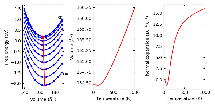
Without plots:

% phonopy-qha e-v.dat thermal_properties.yaml-{-{5..1},{0..5}}

The first argument is the filename of volume-energy data (in the above example, e-v.dat). The volumes and energies are given in \(\text{Angstrom}^3\) and eV, respectively. These energies are only dependent on volume but not on temperature unless using --efe option. Therefore in the simplest case, these are taken as the electronic total energies at 0K. An example of the volume-energy file is:

#   cell volume   energy of cell other than phonon
030000           -42.132246
500000           -42.600974
060000           -42.949142
720000           -43.188162
470000           -43.326751
320000           -43.375124
270000           -43.339884
320000           -43.230619
470000           -43.054343
720000           -42.817825
070000           -42.527932

Lines starting with # are ignored.

The following arguments of phonopy-qha are the filenames of thermal_properties.yaml’s calculated at the volumes given in the volume-energy file. These filenames have to be ordered in the same order as the volumes written in the volume-energy file. Since the volume v.s. free energy fitting is done at each temperature given in thermal_properties.yaml, all thermal_properties.yaml’s have to be calculated in the same temperature ranges and with the same temperature step. phonopy-qha can calculate thermal properties at constant pressure up to the temperature point that is one point less than that in thermal_properties.yaml because of the numerical differentiation with respect to temperature points. Therefore thermal_properties.yaml has to be calculated up to higher temperatures than that expected by phonopy-qha.

Another example for Aluminum is found in the example/Al-QHA directory.

If the condition under pressure is expected, \(PV\) terms may be included in the energies, or equivalent effect is applied using --pressure option.

Experimentally, temperature dependent energies are supported by --efe option. The usage is written at phonopy/phonopy.

Options #

`-h`#

Show help. The available options are shown. Without any option, the results are saved into text files in simple data format.

`--tmax`#

The maximum temperature calculated is specified. This temperature has to be lower than the maximum temperature calculated in thermal_properties.yaml to let at least one temperature points fewer. The default value is --tmax=1000.

`--pressure`#

Pressure is specified in GPa. This corresponds to the \(pV\) term described in the following section Thermal properties in (T, p) space calculated under QHA. Note that bulk modulus obtained with this option than 0 GPa is incorrect.

`-b`#

Fitting volume-energy data to an EOS, and show bulk modulus (without considering phonons). This is made by:

% phonopy-qha -b e-v.dat

`--eos`#

EOS is chosen among vinet, birch_murnaghan, and murnaghan. The default EOS is vinet.

% phonopy-qha --eos='birch_murnaghan' -b e-v.dat

`-p`#

The fitting results, volume-temperature relation, and thermal expansion coefficient are plotted on the display.

`-s`#

The calculated values are written into files.

`--sparse`#

This is used with -s or -p to thin out the number of plots of the fitting results at temperatures. For example with --sparse=10, 1 in 10 temperature curves is only plotted.

`--efe`#

Experimental

Temperature dependent energies other than phonon free energy are included with this option. This is used such as:

% phonopy-qha -p --tmax=1300 --efe fe-v.dat e-v.dat thermal_properties.yaml-{00..10}

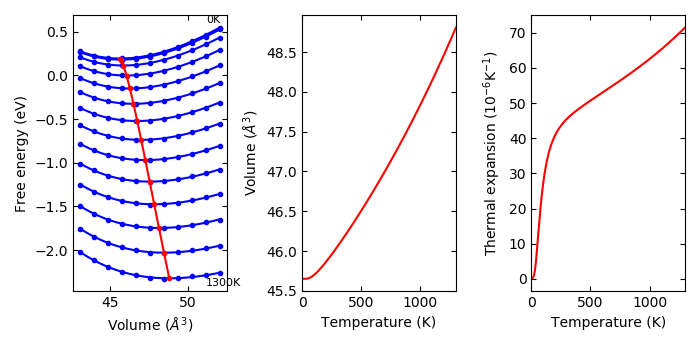
The temperature dependent energies are stored in fe-v.dat. The file format is:

# volume:       43.08047896     43.97798894     44.87549882     45.77300889     46.67051887     47.56802885     48.46553883     49.36304881     50.26055878     51.15806876     52.05557874
#    T(K)     Free energies
    0.0000     -17.27885993    -17.32227490    -17.34336569    -17.34479760    -17.32843604    -17.29673896    -17.25081954    -17.19263337    -17.12356816    -17.04467997    -16.95752155
   10.0000     -17.27886659    -17.32228126    -17.34337279    -17.34481060    -17.32844885    -17.29675204    -17.25083261    -17.19264615    -17.12358094    -17.04469309    -16.95753464
   20.0000     -17.27887453    -17.32228804    -17.34338499    -17.34482383    -17.32846353    -17.29676491    -17.25084547    -17.19265900    -17.12359399    -17.04470709    -16.95754774
...

The first column gives temperatures in K and the following columns give electronic free energies in eV at temperatures and at unit (primitive) cell volumes. The lines starting with # are ignored. This file doesn’t contain the information about cell volumes. Instead, the volumes are obtained from e-v.dat file. The energies in e-v.dat are not used when --efe option is used. The temperature points are expected to be the same as those in thermal_properties.yaml at least up to the maximum temperature specified for phonopy-qha.

An example is given in example/Cu-QHA. The fe-v.dat contains electronic free energy calculated following, e.g., Eqs. (11) and (12) in the paper by Wolverton and Zunger, Phys. Rev. B, 52, 8813 (1994) (of course this paper is not the first one that showed these equations):

\[S_\text{el}(V) = -gk_{\mathrm{B}}\Sigma_i \{ f_i(V) \ln f_i(V) + [1-f_i(V)]\ln [1-f_i(V)] \}\]

with

\[f_i(V) = \left\{ 1 + \exp\left[\frac{\epsilon_i(V) - \mu(V)}{T}\right] \right\}^{-1}\]

and

\[E_\text{el}(V) = g\sum_i f_i(V) \epsilon_i(V),\]

where \(g\) is 1 or 2 for collinear spin polarized and non-spin polarized systems, respectively. For VASP, a script to create fe-v.dat and e-v.dat by these equations is prepared as phonopy-vasp-efe, which is used as:

% phonopy-vasp-efe --tmax=1500 vasprun.xml-{00..10}

where vasprun.xml-{00..10} have to be computed for the same unit cells as those used for thermal_properties.yaml. When phonopy was run with PRIMITIVE_AXES or --pa option, the unit cells for computing electronic eigenvalues have to be carefully chosen to agree with those after applying PRIMITIVE_AXES, or energies are scaled a posteriori.

Note that with --efe, the electronic free energies enter the fitting of \(F(V;T)\) and therefore the equilibrium volumes, thermal expansion, Gibbs free energy, bulk modulus, and Cp-temperature.dat computed by \(-T\partial^2 G/\partial T^2\) include the electronic contributions. However, Cp-temperature_polyfit.dat and gruneisen-temperature.dat are computed from the phonon-only \(C_V\) and \(S\), i.e., the electronic entropy and heat capacity are not included there. Use Cp-temperature.dat for the heat capacity in this case. The Python API (see Electronic free energies from eigenvalues) includes the electronic contributions in both quantities instead.

Output files #

The physical units of V and T are \(\text{Angstrom}^3\) and K, respectively. The unit of eV for Helmholtz and Gibbs energies, J/K/mol for \(C_V\) and entropy, GPa for bulk modulus and pressure are used.

Bulk modulus \(B_T\) (GPa) vs \(T\) (bulk_modulus-temperature.*)
Gibbs free energy \(G\) (eV) vs \(T\) (gibbs-temperature.*)
Heat capacity at constant pressure \(C_p\) (J/K/mol) vs \(T\) computed by \(-T\frac{\partial^2 G}{\partial T^2}\) from three \(G(T)\) points (Cp-temperature.*)
Heat capacity at constant pressure \(C_p\) (J/K/mol) vs \(T\) computed by polynomial fittings of \(C_V(V)\) (Cv-volume.dat) and \(S(V)\) (entropy-volume.dat) for \(\partial S/\partial V\) (dsdv-temperature.dat) and numerical differentiation of \(\partial V/\partial T\), e.g., see Eq.(5) of PRB 81, 174301 by Togo et al. (Cp-temperature_polyfit.*). This may give smoother \(C_p\) than that from \(-T\frac{\partial^2 G}{\partial T^2}\).
Volumetric thermal expansion coefficient \(\beta\) vs \(T\) computed by numerical differentiation (thermal_expansion.*)
Volume vs \(T\) (volume-temperature.*)
Thermodynamics Grüneisen parameter \(\gamma = V\beta B_T/C_V\) (no unit) vs \(T\) (gruneisen-temperature.dat)
Helmholtz free energy (eV) vs volume (helmholtz-volume.*). When --pressure option is specified, energy offset of \(pV\) is added. See also the following section (Thermal properties in (T, p) space calculated under QHA).

Python API: `run_qha`#

Warning

This API is experimental. The function and class names, arguments, and return values described in this section may change in future releases without the usual deprecation process.

phonopy.run_qha is the successor of the deprecated PhonopyQHA class. It takes one Phonopy instance per volume point (with force constants set), computes mesh sampling and thermal properties internally on a given temperature grid, fits the total free energy to an equation of state at each temperature, and returns an immutable QHAResult dataclass. File writers live in phonopy.qha.output and plotting functions in phonopy.qha.plot; both take a QHAResult as the first argument.

import numpy as np
import phonopy
from phonopy import run_qha
from phonopy.qha.output import (
    write_lattice_parameters_temperature,
    write_volume_temperature,
)
from phonopy.qha.plot import plot_qha

phonopys = [phonopy.load(f"phonopy_params-{i:02d}.yaml") for i in range(11)]
internal_energies = np.loadtxt("e-v.dat")[:, 1]  # eV, one per volume
temperatures = np.arange(0, 1101, 10)
result = run_qha(phonopys, temperatures, internal_energies, mesh=100.0)

print(result.equilibrium_volumes)  # V(T)
write_volume_temperature(result)  # volume-temperature.dat
if result.lattice is not None:
    write_lattice_parameters_temperature(result)
plot_qha(result).show()

Remarks:

temperatures must be strictly ascending. One temperature point is consumed by the numerical differentiations, so supply one more point than the temperature range of interest. All temperature-indexed arrays of QHAResult share the same length.
internal_energies are the static internal energies \(U(V)\) other than the phonon free energy in eV with shape (volumes,), e.g., electronic total energies from first-principles calculations or potential energies from machine learning potentials. All energies and volumes of run_qha refer to the primitive cell, to which the phonon thermal properties are normalized. Temperature dependence of the electronic system is supported through electronic_structures (see Electronic free energies from eigenvalues); temperature-dependent free-energy arrays like fe-v.dat are not accepted.
pressure (GPa) and eos (vinet, birch_murnaghan, murnaghan) work as in phonopy-qha.
\(C_p\) is computed by the polynomial-fitting method (see Output files) and is available as result.heat_capacity_P.heat_capacities. The \(-T\partial^2 G/\partial T^2\) variant of the legacy API is not provided.
The file formats written by phonopy.qha.output are identical to those of phonopy-qha for the shared quantities.

Electronic free energies from eigenvalues #

Instead of preparing a fe-v.dat file with phonopy-vasp-efe and the --efe option of phonopy-qha, the same electronic free energies can be computed inside run_qha by supplying the electronic states at each volume point as ElectronicStates (eigenvalues in eV with shape (spin, kpoints, bands), relative k-point weights, and the number of electrons per unit cell):

from phonopy.interface.vasp import parse_vasprunxml
from phonopy.qha.electron import ElectronicStates

electronic_structures = []
for i in range(11):
    vxml = parse_vasprunxml(f"vasprun.xml-{i:02d}")
    electronic_structures.append(
        ElectronicStates(
            eigenvalues=vxml.eigenvalues[:, :, :, 0],
            weights=vxml.k_weights,
            n_electrons=vxml.NELECT,
            volume=vxml.volume[-1],
            internal_energy=vxml.energies[-1, 1],  # energy (sigma -> 0)
        )
    )

result = run_qha(
    phonopys, temperatures, electronic_structures=electronic_structures
)

Since the electronic states carry the volumes and the static internal energies, internal_energies may be omitted (an explicitly given array takes precedence); the volumes are also used for a consistency check against the primitive cell volumes of phonopys.

The electronic free energies \(F_\text{el}(T, V) = U(V) + f_\text{el}(T; V) - f_\text{el}(0; V)\) are computed within the fixed density-of-states (Mermin) approximation with the temperature-dependent chemical potential conserving the number of electrons (see --efe for the equations). This is intended for metals, i.e., the chemical potential is assumed not to lie in a band gap. The electronic entropies are obtained analytically and the electronic heat capacities by a single numerical differentiation; both enter \(C_p\) and the Grüneisen parameters. Note that the deprecated PhonopyQHA computed the Grüneisen parameters with the phonon-only \(C_V\) and \(C_p\) was unavailable in this case, so these quantities differ from the legacy values where the electronic heat capacity is significant. The eigenvalues are not restricted to VASP; any code that provides eigenvalues, k-point weights, and the number of electrons can be used.

For VASP, the collection above can also be done once with

% phonopy-vasp-efe --es vasprun.xml-{00..10}

(--es is short for --write-electronic-states)

which writes electronic_states.hdf5 containing the electronic states together with the volumes and the static energies (sigma->0) of all volume points, instead of computing fe-v.dat. The eigenvalues must be computed for the primitive cell (see the remark on PRIMITIVE_AXES in --efe). The volumes stored with the electronic states are checked against the primitive cell volumes of phonopys by run_qha, which protects against ordering mistakes. The file is loaded with read_electronic_states_hdf5:

from phonopy.qha.electron import read_electronic_states_hdf5

electronic_structures = read_electronic_states_hdf5("electronic_states.hdf5")
result = run_qha(
    phonopys, temperatures, electronic_structures=electronic_structures
)

Lattice parameters a(T), b(T), c(T)#

Note

The setting assumed here is that the structures of the volume series were prepared by relaxing the cell shape under hydrostatic pressures (or equivalently at fixed volumes) using the static total energy only – without the phonon contribution – e.g., by first-principles calculations or machine learning potentials, so that the axial ratios may vary along the volume series, e.g., \(c/a\) of a hexagonal crystal changing with volume. This feature does not optimize \(a\), \(b\), \(c\) with the phonon contribution included: the cell shape at each volume is fixed to the input shape and the phonon free energy optimizes the volume alone, i.e., the cell shape is a function of volume determined by the static total energy. An anisotropic QHA that minimizes \(F(a, b, c;\,T)\) in the full lattice-parameter space is a different calculation and is beyond the scope of this feature.

Since each Phonopy instance carries its unit cell, the lattice parameters at each volume point are known. run_qha propagates their volume dependence to temperature through the equilibrium volumes \(V_0(T)\), giving \(a(T)\), \(b(T)\), \(c(T)\) with generally anisotropic thermal expansion.

The cell volume is modeled as \(V = k\,abc\), where \(a\), \(b\), \(c\) are the lattice-vector lengths of the input unit cells and \(k\) is a geometric constant containing the cell-angle factor. Since \(V\) is the primitive cell volume, \(k\) also absorbs the unit-cell to primitive-cell volume ratio. \(k\) is determined from the input cells and no crystal-system flag is needed: cubic cells simply give constant axial ratios and hexagonal cells give \(b = a\). The axial ratios \(b/a\) and \(c/a\) are fitted as polynomials of \(V\) (degree lattice_fit_degree, default 2), and the lattice parameters are recovered so that \(k\,a(V)\,b(V)\,c(V) = V\) holds exactly. Evaluating them at the equilibrium volumes \(V_0(T)\) gives \(a(T)\), \(b(T)\), \(c(T)\), and the linear thermal expansion coefficients \(\alpha_a = (1/a)\,\mathrm{d}a/\mathrm{d}T\) etc. follow by central differences, satisfying \(\alpha_a + \alpha_b + \alpha_c = \beta\).

The model requires the cell angles to be independent of volume. For triclinic and monoclinic crystals, where cell angles are free parameters, lattice-parameter fitting is therefore skipped with a warning and result.lattice is None (the crystal system is determined from the symmetry of the input cells). In addition, the constancy of \(k\) over the volume points is verified, and the fitting is also skipped when this check fails. This happens when the unit cells are given in a setting whose angles vary with volume even though the crystal system is compatible, for example rhombohedral primitive cells, or fcc primitive cells of a crystal strained along a conventional axis; give the unit cells in a fixed-angle setting such as the conventional cell in such cases.

The results are stored in result.lattice (QHALatticeData): lattice_parameters with shape (temperatures, 3), axial_thermal_expansions with shape (temperatures, 3), k, and ratio_coefficients. The corresponding output files are lattice_parameters-temperature.dat (columns \(T\), \(a\), \(b\), \(c\)) by write_lattice_parameters_temperature and axial_thermal_expansion.dat (columns \(T\), \(\alpha_a\), \(\alpha_b\), \(\alpha_c\), \(\alpha_a+\alpha_b+\alpha_c\)) by write_axial_thermal_expansion. The plotting counterparts are plot_lattice_parameters and plot_axial_thermal_expansion.

Migration from `PhonopyQHA` (deprecated)#

The PhonopyQHA class is deprecated and will be removed in a future major release. The correspondence between the legacy attributes and the new API is:

`PhonopyQHA` (deprecated)	New API
`volume_temperature`	`QHAResult.equilibrium_volumes`
`gibbs_temperature`	`QHAResult.gibbs_free_energies`
`bulk_modulus_temperature`	`QHAResult.bulk_moduli`
`thermal_expansion`	`QHAResult.thermal_expansion`
`heat_capacity_P_polyfit`	`QHAResult.heat_capacity_P.heat_capacities`
`heat_capacity_P_numerical`	not provided (use `heat_capacity_P`)
`gruneisen_temperature`	`QHAResult.gruneisen_parameters`
`helmholtz_volume`	`QHAResult.helmholtz_volume`
`write_*` methods	functions in `phonopy.qha.output`
`plot_*` methods	functions in `phonopy.qha.plot`
`bulk_modulus` (E-V fitting)	`phonopy.qha.core.BulkModulus`

Behavioral differences: run_qha does not accept temperature-dependent electronic free-energy arrays (the fe-v.dat style input of the legacy API); supply electronic_structures instead (see Electronic free energies from eigenvalues). With the electronic contributions included there, QHAResult.gruneisen_parameters and heat_capacity_P differ from the legacy behavior, where the Grüneisen parameters used the phonon-only \(C_V\) and the polyfit \(C_p\) was unavailable.

Thermal properties in (T, p) space calculated under QHA #

Here the word ‘quasi-harmonic approximation’ is used for an approximation that introduces volume dependence of phonon frequencies as a part of anharmonic effect.

A part of temperature effect can be included into total energy of electronic structure through phonon (Helmholtz) free energy at constant volume. But what we want to know is thermal properties at constant pressure. We need some transformation from function of V to function of p. Gibbs free energy is defined at a constant pressure by the transformation:

\[G(T, p) = \min_V \left[ U(V) + F_\mathrm{phonon}(T;\,V) + pV \right],\]

where

\[\min_V[ \text{function of } V ]\]

means to find unique minimum value in the brackets by changing volume. Since volume dependencies of energies in electronic and phonon structures are different, volume giving the minimum value of the energy function in the square brackets shifts from the value calculated only from electronic structure even at 0 K. By increasing temperature, the volume dependence of phonon free energy changes, then the equilibrium volume at temperatures changes. This is considered as thermal expansion under this approximation.

phonopy-qha and run_qha collect the values at volumes and transform them into the thermal properties at constant pressure.

Quasi harmonic approximation

Contents

Quasi harmonic approximation#

-h#

--tmax#

--pressure#

-b#

--eos#

-p#

-s#

--sparse#

--efe#

`-h`#

`--tmax`#

`--pressure`#

`-b`#

`--eos`#

`-p`#

`-s`#

`--sparse`#

`--efe`#