Direct solution of linearized phonon Boltzmann equation

This page explains how to use the direct solution of LBTE by L. Chaput, Phys. Rev. Lett. 110, 265506 (2013) (citation).

How to use

As written in the following sections, this calculation requires large memory space. When running multiple temperature points, simply the memory space needed is multiplied by the number of the temperature points. Therefore it is normally recommended to specify –ts option. An example to run with the direct solution of LBTE for example/Si-PBEsol is as follows:

% phono3py-load --mesh 11 11 11 --lbte --ts 300
...

=================== End of collection of collisions ===================
- Averaging collision matrix elements by phonon degeneracy [0.036s]
- Making collision matrix symmetric (built-in) [0.001s]
----------- Thermal conductivity (W/m-k) with tetrahedron method -----------
Diagonalizing by lapacke dsyev... [0.141s]
Calculating pseudo-inv with cutoff=1.0e-08 (np.dot) [0.001s]
#  T(K)        xx         yy         zz         yz         xz         xy
  300.0     113.140    113.140    113.140      0.000      0.000     -0.000
  (RTA)     108.982    108.982    108.982      0.000      0.000     -0.000
----------------------------------------------------------------------------

Thermal conductivity and related properties were written into
"kappa-m111111.hdf5".
Eigenvalues of collision matrix were written into "coleigs-m111111.hdf5"
...

Memory usage

The direct solution of LBTE needs diagonalization of a large collision matrix, which requires large memory space. This is the largest limitation of using this method. The memory size needed for one collision matrix at a temperature point is \((\text{number of irreducible grid points} \times \text{number of bands} \times 3)^2\) for the symmetrized collision matrix.

These collision matrices contain real values and are supposed to be 64bit float symmetric matrices. During the diagonalization of each collision matrix with LAPACK dsyev solver, around 1.2 times more memory space is consumed in total.

When phono3py runs with –wgp option together with --lbte option, estimated memory space needed for storing collision matrix is presented. An example for example/Si-PBEsol is as follows:

% phono3py-load --mesh 40 40 40 --lbte --wgp
...

Memory requirements:
- Piece of collision matrix at each grid point, temp and sigma: 0.00 Gb
- Full collision matrix at each temp and sigma: 7.15 Gb
- Phonons: 0.04 Gb
- Grid point information: 0.00 Gb
- Phonon properties: 0.14 Gb

...

With –stp option, estimated memory space needed for ph-ph interaction strengths is shown such as

% phono3py-load --mesh 40 40 40 --lbte --stp

Work load distribution

The other difficulty compared with RTA is the workload distribution. Currently there are two ways to distribute the calculation: (1) Collision matrix is divided and the pieces are distributed into computing nodes. (2) Ph-ph interaction strengths at grid points are distributed into computing nodes. These two can not be mixed, so one of them has to be chosen. In either case, the distribution is done simply running a set of phono3py calculations over grid points and optionally band indices. The data computed on each computing node are stored in an hdf5 file. Increasing the calculation size, e.g., larger mesh numbers or larger number of atoms in the primitive cell, large files are created.

Distribution of collision matrix

A full collision matrix is divided into pieces at grid points of irreducible part of Brillouin zone. Each piece is calculated independently from the other pieces. After finishing the calculations of these pieces, the full collision matrix is diagonzalized to obtain the thermal conductivity.

File size of Each piece of the collision matrix can be large. Therefore it is recommended to use –ts option to limit the number of temperature points, e.g., --ts "100 200 300 400 500", depending on the memory size installed on each computing node. To write them into files, --write-collision option must be specified, and to read them from files, --read-collision option is used. These are similarly used as –write-gamma and –read-gamma options for RTA calculation as shown in Workload distribution. --read-collision option collects the pieces and make one full collision matrix, then starts to diagonalize it. This option requires one argument to specify an index to read the collision matrix at one temperature point, e.g., the collision matrix at 200K is read with --read-collision 1 for the (pieces of) collision matrices created with --ts "100 200 300 400 500" (corresponding to 0, 1, 2, 3, 4). The temperature (e.g. 200K) is also read from the file, so it is unnecessary to specify –ts option when reading.

The summary of the procedure is as follows:

1. Running at each grid point with –gp (or –ga) option and saving the piece of the collision matrix to an hdf5 file with --write-collision option. It is probably OK to calculate and store the pieces of the collision matrices at multiple temperatures though it depends on memory size of the computer node. This calculation has to be done at all irreducible grid points.

2. Collecting and creating all necessary pieces of the collision matrix with --read-collision=num (num: index of temperature). By this one full collision matrix at the selected temperature is created and then diagonalized. An option -o num may be used together with --read-collision to distinguish the file names of the results at different temperatures.

Examples of command options are shown below using Si-PBE example. Irreducible grid point indices are obtained by –wgp option:

% phono3py-load --mesh 19 19 19 --lbte --wgp

and the information is given in ir_grid_points.yaml. For distribution of collision matrix calculation (see also Workload distribution):

% phono3py-load --mesh 19 19 19 --lbte --ts 300 --write-collision --gp="grid_point_numbers..."

To collect distributed pieces of the collision matrix:

% phono3py-load --mesh 19 19 19 --lbte --read-collision 0

where --read-collision 0 indicates to read the first result in the list of temperatures by --ts option, i.e., 300K in this case.

Distribution of phonon-phonon interaction strengths

The distribution of pieces of collision matrix is straightforward and is recommended to use if the number of temperature points is small. However increasing data file size, network communication becomes to require long time to send the files from a master node to computation nodes. In this case, the distribution over ph-ph interaction strengths can be another choice. Since, without using –full-pp option, the tetrahedron method or smearing approach with –sigma-cutoff option results in the sparse ph-ph interaction strength data array, i.e., most of the elements are zero, the data size can be reduced by only storing non-zero elements. Not like the collision matrix, the ph-ph interaction strengths in phono3py are independent from temperature though it is not the case if the force constants provided are temperature dependent. Once stored, they are used to create the collision matrices at temperatures. Using --write-pp and --read-pp, they are written into and read from hdf5 files at grid points.

It is also recommended to use –write-phonon option and –read-phonon option to use identical phonon eigenvectors among the distributed nodes.

The summary of the procedure is as follows:

1. Running at each grid point with –gp (or –ga) option and storing the ph-ph interaction strengths to an hdf5 file with --write-pp option. This calculation has to be done at all irreducible grid points.

2. Running with --read-pp option and without –gp (or –ga) option. By this one full collision matrix at the selected temperature is created and then diagonalized. An option -o num may be used together with --read-collision to distinguish the file names of the results at different temperatures.

Examples of command options are shown below using Si-PBE example. Irreducible grid point indices are obtained by –wgp option

% phono3py-load --mesh "19 19 19" --lbte --wgp

and the grid point information is provided in ir_grid_points.yaml. All phonons on mesh grid points are saved by

% phono3py-load --mesh "19 19 19" --write-phonon

For distribution of ph-ph interaction strength calculation (see also Workload distribution)

% phono3py-load --mesh "19 19 19" --lbte --ts 300 --write-pp --gp "grid_point_numbers..." --read-phonon

Here one temperature has to be specified but any one of temperatures is OK since ph-ph interaction strength computed here is assumed to be temperature independent. Then the computed ph-ph interaction strengths are read and used to compute collision matrix and lattice thermal conductivity at a temperature by

% phono3py-load --mesh "19 19 19" --lbte --ts 300 --read-pp --read-phonon

This last command is repeated at different temperatures to obtain the properties at multiple temperatures.

Cutoff parameter of pseudo inversion

To achieve a pseudo inversion, a cutoff parameter is used to find null space, i.e., to select the nearly zero eigenvalues. The default cutoff value is 1e-8, and this hopefully works in many cases. But if a collision matrix is numerically not very accurate, we may have to carefully choose the value by --pinv-cutoff option. It is safer to plot the absolute values of eigenvalues in log scale to see if there is clear gap between non-zero eigenvalue and nearly-zero eigenvalues. After running the direct solution of LBTE, coleigs-mxxx.hdf5 is created. This contains the eigenvalues of the collision matrix (either symmetrized or non-symmetrized). The eigenvalues are plotted using phono3py-coleigplot in the phono3py package:

% phono3py-coleigplot coleigs-mxxx.hdf5

It is assumed that only one set of eigenvalues at a temperature point is contained.

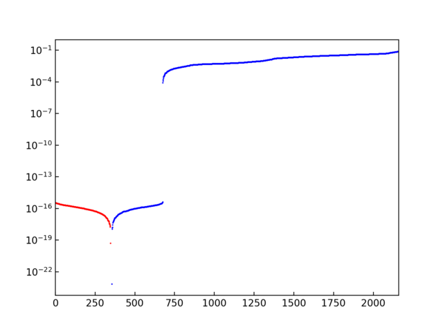
Eigenvalues are plotted in log scale (Si-PBEsol exmaple with 15x15x15 mesh). The number in x-axis is just the index where each eigenvalue is stored. Normally the eigenvalues are stored ascending order. The bule points show the positive values, and the red points show the negative values as positive values (absolute values) to be able to plot in log scale. In this plot, we can see the gap between \(10^{-4}\) and \(10^{-16}\), which is a good sign. The values whose absolute values are smaller than \(10^{-8}\) are treated as 0 and those solutions are considered as null spaces.

Diagonalization solver interfaces

Multithreaded BLAS is recommended to use for the calculation of the direct solution of LBTE because the diagonalization of the collision matrix is computationally highly demanding. The diagonalization in Phono3py relies on LAPACK via BLAS library. There are choices of the BLAS libraries. OpenBLAS and MKL are considered most popular choices. For non-INTEL (or AMD) systems such as ARM64, MKL can not be used. How to choose the BLAS library in installation via conda-forge is written here.

Phono3py has two different interfaces to the LAPACK library. One is via scipy (or numpy), and the other is via LAPACKE as shown below. How to switch between interfaces is described in the next section.

OpenBLAS or MKL linked scipy and numpy

Scipy and numpy have interfaces to LAPACK dsyevd, and scipy also has the interface to dsyev. OpenBLAS and MKL linked scipy and numpy are provided by conda-forge.

OpenBLAS or MKL via LAPACKE

LAPACK dsyev and dsyevd can be accessed via LAPACKE in the phono3py’s C language implementation through the python C-API.

Solver choice for diagonalization

For larger systems, diagonalization of collision matrix takes longest time and requires large memory space. Phono3py relies on LAPACK for the diagonalization and so the performance is dependent on the choice of the diagonalization solver.

Using multithreaded BLAS with many-core computing node, computing time may be well reduced and the calculation can finish in a realistic time. Currently scipy, numpy and LAPACKE can be used as the LAPACK wrapper in phono3py. Scipy and numpy distributed by anaconda are MKL linked, therefore MKL multithread BLAS is used through them. Multithreaded OpenBLAS is installed by conda and can be used via LAPACKE in phono3py. MKL LAPACK and BLAS are also able to be used via LAPACKE in phono3py with appropriate setting in setup.py.

Using --pinv-solver=[number], one of the following solver is chosen:

1. Lapacke dsyev: Smaller memory consumption than dsyevd, but slower. This is the default solver when MKL LAPACKE is integrated or scipy is not installed.

2. Lapacke dsyevd: Larger memory consumption than dsyev, but faster. This is not considered as stable as dsyev but can be significantly faster than dsyev for solving large collision matrix. It is recommended to compare the result with that by dsyev solver using smaller collision matrix (e.g., sparser sampling mesh) before starting solving large collision matrix.

3. Numpy’s dsyevd (linalg.eigh). Similar to solver (2), this solver should be used carefully.

4. Scipy’s dsyev: This is the default solver when scipy is installed and MKL LAPACKE is not integrated.

5. Scipy’s dsyevd: Similar to solver (2), this solver should be used carefully.