Auxiliary tools

phono3py-kaccum: Cumulative lattice thermal conductivity and related properties

Cumulative physical properties with respect to frequency or mean free path are calculated using this command.

For example, cumulative thermal conductivity is defined by

\[ \kappa^\text{c}(\omega) = \int^\omega_0 \frac{1}{N} \sum_\lambda \kappa_\lambda \delta(\omega_\lambda - \omega') d\omega' \]

\(\kappa_\lambda\) is the contribution to \(\kappa\) from the phonon mode \(\lambda\), which is defined as

\[ \kappa_\lambda = \frac{1}{V_0} C_\lambda \mathbf{v}_\lambda \otimes \mathbf{v}_\lambda \tau_\lambda. \]

(The notations are found in http://arxiv.org/abs/1501.00691.)

How to use phono3py-kaccum

Let’s compute lattice thermal conductivity of Si using the Si-PBEsol example found in the example directory.

% phono3py --mesh="11 11 11" --sym-fc --br

Then using the output file, kappa-m111111.hdf5, run phono3py-kaccum as follows:

% phono3py-kaccum kappa-m111111.hdf5 |tee kaccum.dat

kappa-m111111.hdf5 is the output file of thermal conductivity calculation, which is passed to phono3py-kaccum as the first argument. phono3py_disp.yaml or phono3py.yaml is necessary to be located under the current directory to read the crystal structure.

The format of the output is as follows: The first column gives frequency in THz, and the second to seventh columns give the cumulative lattice thermal conductivity of 6 elements, xx, yy, zz, yz, xz, xy. The eighth to 13th columns give the derivatives. There are sets of frequencies, which are separated by blank lines. Each set is for a temperature. There are the groups corresponding to the number of temperatures calculated.

To plot the output by gnuplot at temperature index 30 that may correspond to 300 K,

% gnuplot
...
gnuplot> p "kaccum.dat" i 30 u 1:2 w l, "kaccum.dat" i 30 u 1:8 w l

The plot like below is displayed.

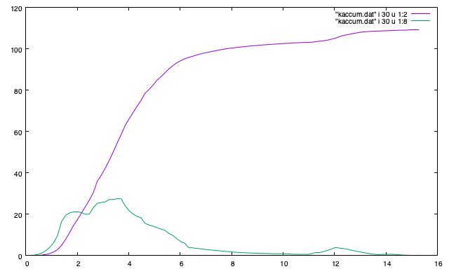
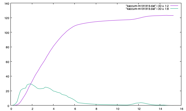
With \(19\times 19\times 19\) mesh:

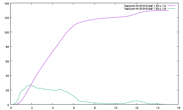
That calculated by QE with \(19\times 19\times 19\) mesh:

General options

--temperature

Pick up one temperature point. For example, --temperature=300 for 300 K, which works only if thermal conductivity is calculated at temperatures including 300 K.

--nsp

Number of points to be sampled in the x-axis.

Options for tensor properties

For cummulative thermal conductivity, the last value is given as the thermal conductivity in W/mK. For the other properties, the last value is effectively the sum of values on all mesh grids divided by number of mesh grids. This is understood as normalized for one primitive cell. Before version 1.11.13.1, the last value for gv_by_gv (–gv option) was further divided by the primitive cell volume.

Number of columns of output data is 13 as explained above. With --average and --trace options, number of columns of output data becomes 3.

--mfp

Mean free path (MFP) is used instead of frequency for the x-axis. MFP is defined in the single-mode RTA by a vector

\[ \mathbf{l}_\lambda = \mathbf{v}_\lambda \tau_\lambda. \]

The MFP cumulative \(\kappa^\text{c}(l)\) is given by

\[ \kappa^\text{c}(l) = \int^l_0 \frac{1}{N} \sum_\lambda \kappa_\lambda \delta(l_\lambda - l') dl' \]

where \(l_\lambda = |\mathbf{l}_\lambda|\) and \(\kappa_\lambda\) is the contribution to \(\kappa\) from the phonon mode \(\lambda\) in the single-mode RTA, which is defined as

\[ \kappa_\lambda = \frac{1}{V_0} C_\lambda \mathbf{v}_\lambda \otimes \mathbf{v}_\lambda \tau_\lambda = \frac{1}{V_0} C_\lambda \mathbf{v}_\lambda \otimes \mathbf{l}_\lambda. \]

The physical unit of MFP is Angstrom.

The figure below shows the results of Si example with the \(19\times 19\times 19\) and \(11\times 11\times 11\) sampling meshes used for the lattice thermal conductivity calculation. They look differently. Especially for the result of the \(11\times 11\times 11\) sampling mesh, the MFP seems converging but we can see it’s not true to look at that of the \(19\times 19\times 19\) sampling mesh. To show this type of plot, be careful about the sampling mesh convergence.

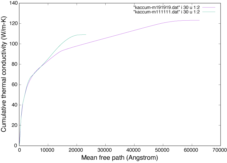
(This plot is based on the Si-PBEsol example.)

--gv

Outer product of group velocities \(\mathbf{v}_\lambda \otimes \mathbf{v}_\lambda\) divided by primitive cell volume (in \(\text{THz}^2 / \text{Angstrom}\)).

--average

Output the traces of the tensors divided by 3 rather than the unique elements.

--trace

Output the traces of the tensors rather than the unique elements.

Options for scalar properties

For the following properties, those values are normalized by the number of full grid points. This is understood as normalized for one primitive cell.

Number of columns of output data is three, frequency, cumulative property, and derivative of cumulative property such like DOS.

--gamma

\(\Gamma_\lambda(\omega_\lambda)\) (in THz).

--tau

Lifetime \(\tau_\lambda = \frac{1}{2\Gamma_\lambda(\omega_\lambda)}\) (in ps)

--cv

Modal heat capacity \(C_\lambda\) (in eV/K).

--gv-norm

Absolute value of group velocity \(|\mathbf{v}_\lambda|\) (in \(\text{THz}\cdot\text{Angstrom}\)).

--pqj

Averaged phonon-phonon interaction \(P_{\mathbf{q}j}\) (in \(\text{eV}^2\)).

--dos

Constant value of 1. This results in phonon DOS.

phono3py-kdeplot: Distribution of phonon lifetime

This script is under the development and may contain bugs. But a feature is briefly introduced below since it may be useful. Scipy is needed to use this script.

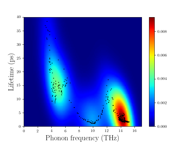
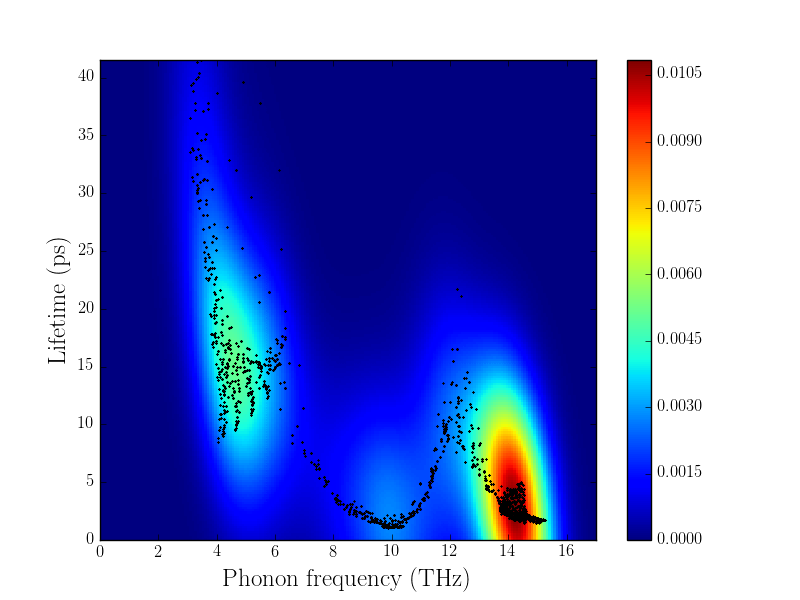
This script draws density of phonon modes in the frequency-lifetime plane. Its density is estimated using Gaussian-KDE using scipy. Then (frequency, lifetime)-data points are superimposed on the density plot.

phono3py-kdeplot reads a result of the thermal conductivity calculation as the first argument:

% phono3py-kdeplot kappa-m111111.hdf5

This calculation takes some time from minutes to hours depending on mesh numbers and nbins. Therefore it is recommended to start with smaller mesh and gradually to increase mesh numbers and nbins up to satisfaction.

After finishing the calculation, the plot is saved in lifetime.png. The black dots show original data points. The drawing area is automatically set to make the look good, where its higher lifetime side is not drawn if all density beyond a lifetime value is smaller than some ratio (see --dr, --density-ratio) of the maximum density.

The following plot is drawn with a \(19 \times 19 \times 19\) mesh and nbins=200 and the Si-PBEsol example is used to generate the data. The colormap of ‘jet’ in matplotlib is used.

Options

--temperature

Pick up one temperature point. For example, --temperature=300 for 300 K, which works only if thermal conductivity is calculated at temperatures including 300 K.

Without specifying this option, the 31st temperature index is chosen. This often corresponds to 300 K if phono3py ran without setting temperature range and step.

--nbins

This option controls the resolution of the density plot. The default value is 100. With larger nbins, the resolution of the plot becomes better, but the computation will take more time.

% phono3py-kdeplot --nbins=200 kappa-m111111.hdf5

--cutoff, --fmax

The option --cutoff (--fmax) sets the maximum value of lifetime (frequency) to be included as data points before Gaussian-KDE. Normally increasing this value from the chosen value without specifying this option does nothing since automatic control of drawing area cuts high lifetime (frequency) side if the density is low.

--xmax and --ymax

Maximum values of drawing region of phonon frequency (x-axis) and lifetime (y-axis) are specified by --xmax and --ymax, respectively.

--ymax switches off automatic determination of maximum value of drawing region along y-axis, therefore as a side effect, the computation will be roughly twice faster.

% phono3py-kdeplot --ymax=60 kappa-m111111.hdf5

--zmax

Maximum value of the density is specified with this option. The color along colorbar saturates by choosing a smaller value than the maximum value of density in the data.

--dr, --density-ratio

The density threshold is specified by the ratio with respect to maximum density. Normally smaller value results in larger drawing region. The default value is 0.1. When --ymax is specified together, this option is ignored.

% phono3py-kdeplot --dr=0.01 kappa-m111111.hdf5

--cmap

Color map to be used for the density plot. It’s given by the name presented at the matplotlib documentation, https://matplotlib.org/users/colormaps.html. The default colormap depends on your matplotlib environment.

% phono3py-kdeplot --cmap="OrRd" kappa-m111111.hdf5

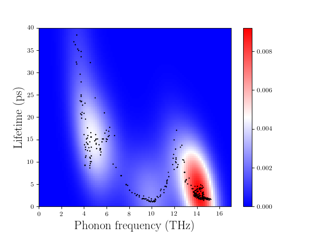
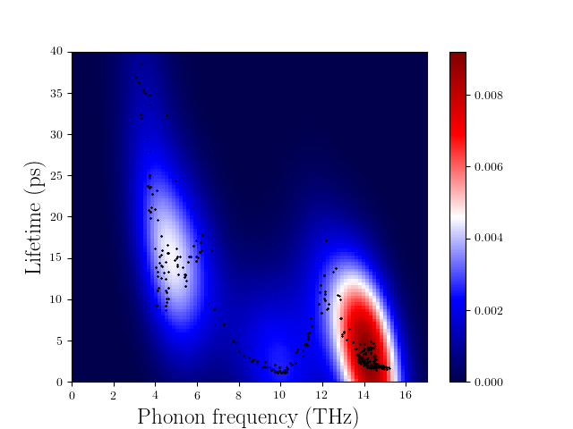
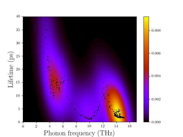
The following figures are those drawn with jet, bwr, seismic, gnuplot, hsv, and OrRd colormaps.