Command options / Setting tags

Phono3py is operated with command options or with a configuration file that contains setting tags. In this page, the command options are explained. Most of command options have their respective setting tags.

A configuration file with setting tags like phonopy can be used instead of and together with the command options. The setting tags are mostly equivalent to the respective most command options, but when both are set simultaneously, the command options are preferred. An example of configuration (e.g., saved in a file setting.conf) is as follow:

DIM = 2 2 2
DIM_FC2 = 4 4 4
PRIMITIVE_AXES = 0 1/2 1/2 1/2 0 1/2 1/2 1/2 0
MESH = 11 11 11
BTERTA = .TRUE.
NAC = .TRUE.
READ_FC2 = .TRUE.
READ_FC3 = .TRUE.
CELL_FILENAME = POSCAR-unitcell

where the setting tag names are case insensitive. This is run by

% phono3py setting.conf [comannd options]

or

% phono3py [comannd options] -- setting.conf

Input cell file name

-c (CELL_FILENAME)

This specifies input unit cell filename.

% phono3py -c POSCAR-unitcell ... (many options)

Calculator interface

--qe (CALCULATOR = QE)

Quantum espresso (pw) interface is invoked. See the detail at Quantum ESPRESSO (pw) & phono3py calculation.

--crystal (CALCULATOR = CRYSTAL)

CRYSTAL interface is invoked. See the detail at CRYSTAL & phono3py calculation.

--turbomole (CALCULATOR = TURBOMOLE)

TURBOMOLE interface is invoked. See the details at TURBOMOLE & phono3py calculation.

Utilities to create default input files

These options have no respective configuration file tags.

--cf3 (command option only)

This is used to create FORCES_FC3 from disp_fc3.yaml and force calculator outputs containing forces in supercells. disp_fc3.yaml has to be located at the current directory. Calculator interface has to be specified except for VASP (default) case.

% phono3py --cf3 disp-{00001..00755}/vasprun.xml

% phono3py --qe --cf3 supercell_out/disp-{00001..00111}/Si.out

--cf3-file (command option only)

This is used to create FORCES_FC3 from a text file containing a list of calculator output file names. disp_fc3.yaml has to be located at the current directory. Calculator interface has to be specified except for VASP (default) case.

% phono3py --cf3-file file_list.dat

where file_list.dat contains file names that can be recognized from the current directory and is expected to be like:

disp-00001/vasprun.xml
disp-00002/vasprun.xml
disp-00003/vasprun.xml
disp-00004/vasprun.xml
...

The order of the file names is important. This option may be useful to be used together with --cutoff-pair option.

--cf2 (command option only)

This is used to create FORCES_FC2 similarly to --cf3 option. disp_fc2.yaml has to be located at the current directory. This is optional. Calculator interface has to be specified except for VASP (default) case. FORCES_FC2 is necessary to run with --dim-fc2 option.

% phono3py --cf2 disp_fc2-{00001..00002}/vasprun.xml

--cfz (command option only)

This is used to create FORCES_FC3 and FORCES_FC2 subtracting residual forces combined with --cf3 and --cf2, respectively. Calculator interface has to be specified except for VASP (default) case.

In the following example, it is supposed that disp3-00000/vasprun.xml and disp2-00000/vasprun.xml contain the forces of the perfect supercells. In ideal case, these forces are zero, but often they are not. Here, this is called “residual forces”. Sometimes quality of force constants is improved in this way.

% phono3py --cf3 disp3-{00001..01254}/vasprun.xml --cfz disp3-00000/vasprun.xml
% phono3py --cf2 disp2-{00001..00006}/vasprun.xml --cfz disp2-00000/vasprun.xml

--fs2f2 or --force-sets-to-forces-fc2 (command option only)

FORCES_FC2 and disp_fc2.yaml are created from phonopy’s FORCE_SETS file.

% phono3py --fs2f2

--cfs or --create-force-sets (command option only)

Phonopy’s FORCE_SETS is created from FORCES_FC3 and disp_fc3.yaml.

% phono3py --cfs

In conjunction with –dim-fc2, phonopy’s FORCE_SETS is created from FORCES_FC2 and disp_fc2.yaml instead of FORCES_FC3 and disp_fc3.yaml.

% phono3py --cfs --dim-fc2="x x x"

Supercell and primitive cell

--dim (DIM)

Supercell dimension is specified. See the detail at http://phonopy.github.io/phonopy/setting-tags.html#dim .

--dim-fc2 (DIM_FC2)

Supercell dimension for 2nd order force constants (for harmonic phonons) is specified. This is optional.

A larger and different supercell size for 2nd order force constants than that for 3rd order force constants can be specified with this option. Often interaction between a pair of atoms has longer range in real space than interaction among three atoms. Therefore to reduce computational demand, choosing larger supercell size only for 2nd order force constants may be a good idea.

Using this option with -d option, the structure files (e.g. POSCAR_FC2-xxxxx or equivalent files for the other interfaces) and disp_fc2.yaml are created. These are used to calculate 2nd order force constants for the larger supercell size and these force calculations have to be done in addition to the usual force calculations for 3rd order force constants.

phono3py -d --dim="2 2 2" --dim-fc2="4 4 4" -c POSCAR-unitcell

After the force calculations, --cf2 option is used to create FORCES_FC2.

phono3py --cf2 disp-{001,002}/vasprun.xml

To calculate 2nd order force constants for the larger supercell size, FORCES_FC2 and disp_fc2.yaml are necessary. Whenever running phono3py for the larger 2nd order force constants, --dim-fc2 option has to be specified. fc2.hdf5 created as a result of running phono3py contains the 2nd order force constants with larger supercell size. The filename is the same as that created in the usual phono3py run without --dim-fc2 option.

phono3py --dim="2 2 2" --dim_fc2="4 4 4" -c POSCAR-unitcell ... (many options)

--pa, --primitive-axes (PRIMITIVE_AXES)

Transformation matrix from a non-primitive cell to the primitive cell. See phonopy PRIMITIVE_AXES tag (--pa option) at http://phonopy.github.io/phonopy/setting-tags.html#primitive-axis

Displacement creation

-d (CREATE_DISPLACEMENTS = .TRUE.)

Supercell with displacements are created. Using with --amplitude option, atomic displacement distances are controlled. With this option, files for supercells with displacements and disp_fc3.yaml file are created.

--amplitude (DISPLACEMENT_DISTANCE)

Atomic displacement distance is specified. This value may be increased for the weak interaction systems and descreased when the force calculator is numerically very accurate.

The default value depends on calculator. See Default displacement distance created.

Force constants

--cfc or --compact-fc (COMPACT_FC = .TRUE.)

When creating force constants from FORCES_FC3 and/or FORCES_FC2, force constants that use smaller data size are created. The shape of the data array is (num_patom, num_satom) for fc2 and (num_patom, num_satom, num_satom) for fc3, where num_patom and num_satom are the numbers of atoms in primtive cell and supercell. In the full size force constants case, num_patom is replaced by num_satom. Therefore if the supercell dimension is large, this reduction of data size becomes large. If the input crystal structure has centring –pa is necessary to have smallest data size. In this case, --pa option has to be specified on reading. Otherwise phono3py can recognize if fc2.hdf5 and fc3.hdf5 are compact or full automatically. When using with --sym-fc, the calculated results will become slightly different due to imperfect symmetrization scheme that phono3py employs.

% phono3py --dim="2 2 2" --cfc --pa="0 1/2 1/2 1/2 0 1/2 1/2 1/2 0" -c POSCAR-unitcell

--sym-fc (FC_SYMMETRY = .TRUE.)

Second- and third-order force constants are symmetrized. The index exchange of real space force constantsand translational invariance symmetry are applied in a simple way. This symmetrization just removes drift force constants evenly from all elements and then applies averaging index-exchange equivalent elements. Therefore the different symmetries are not simultaneously enforced. For better symmetrization, it is recommended to use an external force constants calculator like ALM.

The symmetrizations for the second and third orders can be independently applied by --sym-fc2 (SYMMETRIZE_FC2 = .TRUE.) and --sym-fc3r (SYMMETRIZE_FC3 = .TRUE.), , respectively.

--cutoff-fc3 or --cutoff-fc3-distance (CUTOFF_FC3_DISTANCE)

This option is not used to reduce number of supercells with displacements, but this option is used to set zero in elements of given third-order force constants. The zero elements are selected by the condition that any pair-distance of atoms in each atom triplet is larger than the specified cut-off distance.

If one wants to reduce number of supercells, the first choice is to reduce the supercell size and the second choice is using --cutoff-pair option.

--cutoff-pair or --cutoff-pair-distance (CUTOFF_PAIR_DISTANCE)

This option is only used together with -d option.

A cutoff pair-distance in a supercell is used to reduce the number of necessary supercells with displacements to obtain third order force constants. As the drawback, a certain number of third-order-force-constants elements are abandoned or computed with less numerical accuracy. More details are found in the following link:

• Force constants calculation with cutoff pair-distance

Reciprocal space sampling mesh and grid points, and band indices

--mesh (MESH or MESH_NUMBERS)

Mesh sampling grids in reciprocal space are generated with the specified numbers. This mesh is made along reciprocal axes and is always Gamma-centered. Except for that this mesh is always Gamma-centered, this works in the same way as written here, https://phonopy.github.io/phonopy/setting-tags.html#mesh-mp-or-mesh-numbers.

--gp (GRID_POINTS)

Grid points are specified by their unique indices, e.g., for selecting the q-points where imaginary parts of self energees are calculated. For thermal conductivity calculation, this can be used to distribute its calculation over q-points (see Workload distribution).

Indices of grid points are specified by space or comma (,) separated numbers. The mapping table between grid points to its indices is obtained by running with --loglevel=2 option.

% phono3py --dim="2 2 2" --pa="0 1/2 1/2 1/2 0 1/2 1/2 1/2 0" -c POSCAR-unitcell --mesh="19 19 19" --fc3 --fc2 --br --write-gamma --gp="0 1 2 3 4 5"

where --gp="0 1 2 3 4 5" can be also written --gp="0,1,2,3,4,5". --ga option below can be used similarly for the same purpose.

--ga (GRID_ADDRESSES)

This is used to specify grid points like --gp option but in their addresses represented by integer numbers. For example with --mesh="16 16 16", a q-point of (0.5, 0.5, 0.5) is given by --ga="8 8 8". The values have to be integers. If you want to specify the point on a path, --ga="0 0 0 1 1 1 2 2 2 3 3 3 ...", where each three values are recogninzed as a grid point. The grid points given by --ga option are translated to grid point indices as given by --gp option, and the values given by --ga option will not be shown in log files.

--bi (BAND_INDICES)

Band indices are specified. The output file name will be, e.g., gammas-mxxx-gxx(-sx)-bx.dat where bxbx... shows the band indices used to be averaged. The calculated values at indices separated by space are averaged, and those separated by comma are separately calculated.

% phono3py --fc3 --fc2 --dim="2 2 2" --mesh="16 16 16" -c POSCAR-unitcell --nac --gp="34" --bi="4 5, 6"

This may be also useful to distribute the computational demand such like that the unit cell is large and the calculation of phonon-phonon interaction is heavy.

--wgp (command option only)

Irreducible grid point indices and related information are written into ir_grid_points.yaml. This information may be used when we want to distribute thermal conductivity calculation into small pieces or to find specific grid points to calculate imaginary part of self energy, for which –gp option can be used to specify the grid point indices.

grid_address-mxxx.hdf5 is also written. This file contains all the grid points and their grid addresses in integers. Q-points corresponding to grid points are calculated divided these integers by sampling mesh numbers for respective reciprocal axes.

% phono3py --dim="2 2 2" --pa="0 1/2 1/2 1/2 0 1/2 1/2 1/2 0" -c POSCAR-unitcell --mesh="19 19 19" --wgp

--stp (command option only)

Numbers of q-point triplets to be calculated for irreducible grid points for specified sampling mesh numbers are shown. This can be used to estimate how large a calculation is. Only those for specific grid points are shown by using with --gp or --ga option.

% phono3py --dim="2 2 2" --pa="0 1/2 1/2 1/2 0 1/2 1/2 1/2 0" -c POSCAR-unitcell --mesh="19 19 19" --stp --gp 20

Brillouin zone integration

--thm (TETRAHEDRON = .TRUE.)

Tetrahedron method is used for calculation of imaginary part of self energy. This is the default option. Therefore it is not necessary to specify this unless both results by tetrahedron method and smearing method in one time execution are expected.

--sigma (SIGMA)

\(\sigma\) value of Gaussian function for smearing when calculating imaginary part of self energy. See the detail at Brillouin zone summation.

Multiple \(\sigma\) values are also specified by space separated numerical values. This is used when we want to test several \(\sigma\) values simultaneously.

--sigma-cutoff (SIGMA_CUTOFF_WIDTH)

The tails of the Gaussian functions that are used to replace delta functions in the equation shown at –full-pp are cut with this option. The value is specified in number of standard deviation. --sigma-cutoff=5 gives the Gaussian functions to be cut at \(5\sigma\). Using this option scarifies the numerical accuracy. So the number has to be carefully tested. But computation of phonon-phonon interaction strength becomes much faster in exchange for it.

--full-pp (FULL_PP = .TRUE.)

For thermal conductivity calculation using the linear tetrahedron method (from version 1.10.5) and smearing method with --simga-cutoff (from version 1.12.3), only necessary elements (i.e., that have non-zero delta functions) of phonon-phonon interaction strength, \(\bigl|\Phi_{-\lambda\lambda'\lambda''}\bigl|^2\), is calculated due to delta functions in calculation of \(\Gamma_\lambda(\omega)\),

\[\Gamma_\lambda(\omega) = \frac{18\pi}{\hbar^2} \sum_{\lambda' \lambda''} \bigl|\Phi_{-\lambda\lambda'\lambda''}\bigl|^2 \left\{(n_{\lambda'}+ n_{\lambda''}+1) \delta(\omega-\omega_{\lambda'}-\omega_{\lambda''}) \right. + (n_{\lambda'}-n_{\lambda''}) \left[\delta(\omega+\omega_{\lambda'}-\omega_{\lambda''}) - \left. \delta(\omega-\omega_{\lambda'}+\omega_{\lambda''}) \right]\right\}.\]

But using this option, full elements of phonon-phonon interaction strength are calculated and averaged phonon-phonon interaction strength (\(P_{\mathbf{q}j}\), see –ave-pp) is also given and stored.

Method to solve BTE

--br (BTERTA = .TRUE.)

Run calculation of lattice thermal conductivity tensor with the single mode relaxation time approximation (RTA) and linearized phonon Boltzmann equation. Without specifying --gp (or --ga) option, all necessary phonon lifetime calculations for grid points are sequentially executed and then thermal conductivity is calculated under RTA. The thermal conductivity and many related properties are written into kappa-mxxx.hdf5.

With --gp (or --ga) option, phonon lifetimes on the specified grid points are calculated. To save the results, --write-gamma option has to be specified and the physical properties belonging to the grid points are written into kappa-mxxx-gx(-sx).hdf5.

--lbte (LBTE = .TRUE.)

Run calculation of lattice thermal conductivity tensor with a direct solution of linearized phonon Boltzmann equation. The basis usage of this option is equivalent to that of --br. More detail is documented at Direct solution of linearized phonon Boltzmann equation.

Scattering

--isotope (ISOTOPE =.TRUE.)

Phonon-isotope scattering is calculated based on the formula by Shin-ichiro Tamura, Phys. Rev. B, 27, 858 (1983). Mass variance parameters are read from database of the natural abundance data for elements, which refers Laeter et al., Pure Appl. Chem., 75, 683 (2003).

% phono3py --dim="3 3 2" -v --mesh="32 32 20" -c POSCAR-unitcell --br --isotope

--mass-variances or --mv (MASS_VARIANCES)

Mass variance parameters are specified by this option to include phonon-isotope scattering effect in the same way as --isotope option. For example of GaN, this may be set like --mv="1.97e-4 1.97e-4 0 0". The number of elements has to correspond to the number of atoms in the primitive cell.

Isotope effect to thermal conductivity may be checked first running without isotope calculation:

% phono3py --dim="3 3 2" -v --mesh="32 32 20" -c POSCAR-unitcell --br

Then running with isotope calculation:

% phono3py --dim="3 3 2" -v --mesh="32 32 20" -c POSCAR-unitcell --br --read-gamma --mv="1.97e-4 1.97e-4 0 0"

In the result hdf5 file, currently isotope scattering strength is not written out, i.e., gamma is still imaginary part of self energy of ph-ph scattering.

--boundary-mfp, --bmfp (BOUNDARY_MFP)

A most simple phonon boundary scattering treatment is included. \(v_g/L\) is just used as the scattering rate, where \(v_g\) is the group velocity and \(L\) is the boundary mean free path. The value is given in micrometre. The default value, 1 metre, is just used to avoid divergence of phonon lifetime and the contribution to the thermal conducitivity is considered negligible.

--ave-pp (USE_AVE_PP = .TRUE.)

Averaged phonon-phonon interaction strength (\(P_{\mathbf{q}j}=P_\lambda\)) is used to calculate imaginary part of self energy in thermal conductivity calculation. \(P_\lambda\) is defined as

\[P_\lambda = \frac{1}{(3n_\text{a})^2}\sum_{\lambda' \lambda''}|\Phi_{\lambda \lambda' \lambda''}|^2,\]

where \(n_\text{a}\) is the number of atoms in unit cell. This is roughly constant with respect to the sampling mesh density for converged \(|\Phi_{\lambda \lambda' \lambda''}|^2\). Then for all \(\mathbf{q}',j',j''\),

\[|\Phi_{\mathbf{q}j,\mathbf{q}'j',\mathbf{G-q-q'}j''}|^2 := P_{\mathbf{q}j} / N,\]

where \(N\) is the number of grid points on the sampling mesh. \(\Phi_{\lambda \lambda' \lambda''} \equiv 0\) unless \(\mathbf{q} + \mathbf{q}' + \mathbf{q}'' = \mathbf{G}\).

This option works only when --read-gamma and --br options are activated where the averaged phonon-phonon interaction that is read from kappa-mxxx(-sx-sdx).hdf5 file is used if it exists in the file. Therefore the averaged phonon-phonon interaction has to be stored before using this option (see –full-pp). The calculation result overwrites kappa-mxxx(-sx-sdx).hdf5 file. Therefore to use this option together with -o option is strongly recommended.

First, run full conductivity calculation,

% phono3py --dim="3 3 2" -v --mesh="32 32 20" -c POSCAR-unitcell --br

Then

% phono3py --dim="3 3 2" -v --mesh="32 32 20" -c POSCAR-unitcell --br --read-gamma --ave-pp -o ave_pp

--const-ave-pp (CONST_AVE_PP = .TRUE.)

Averaged phonon-phonon interaction (\(P_{\mathbf{q}j}\)) is replaced by this constant value and \(|\Phi_{\lambda \lambda' \lambda''}|^2\) are set as written in –ave-pp for thermal conductivity calculation. This option works only when --br options are activated. Therefore third-order force constants are not necessary to input. The physical unit of the value is \(\text{eV}^2\).

% phono3py --dim="3 3 2" -v --mesh="32 32 20" -c POSCAR-unitcell --br --const-ave-pp=1e-10

--nu (N_U = .TRUE.)

Integration over q-point triplets for the calculation of \(\Gamma_\lambda(\omega_\lambda)\) is made separately for normal \(\Gamma^\text{N}_\lambda(\omega_\lambda)\) and Umklapp \(\Gamma^\text{U}_\lambda(\omega_\lambda)\) processes. The sum of them is usual \(\Gamma_\lambda(\omega_\lambda) = \Gamma^\text{N}_\lambda(\omega_\lambda) + \Gamma^\text{U}_\lambda(\omega_\lambda)\) and this is used to calcualte thermal conductivity in single-mode RTA. The separation, i.e., the choice of G-vector, is made based on the first Brillouin zone.

The data are stored in kappa-mxxx(-gx-sx-sdx).hdf5 file and accessed by gamma_N and gamma_U keys. The shape of the arrays is the same as that of gamma (see gamma). An example (Si-PBEsol) is shown below:

% phono3py --dim="2 2 2" --pa="0 1/2 1/2 1/2 0 1/2 1/2 1/2 0" -c POSCAR-unitcell --mesh="11 11 11" --fc3 --fc2 --br --nu
...
% ipython

In [1]: import h5py

In [2]: f = h5py.File("kappa-m111111.hdf5", 'r')

In [3]: list(f)
Out[3]:
['frequency',
 'gamma',
 'gamma_N',
 'gamma_U',
 'group_velocity',
 'gv_by_gv',
 'heat_capacity',
 'kappa',
 'kappa_unit_conversion',
 'mesh',
 'mode_kappa',
 'qpoint',
 'temperature',
 'weight']

In [4]: f['gamma'].shape
Out[4]: (101, 56, 6)

In [5]: f['gamma_N'].shape
Out[5]: (101, 56, 6)

In [6]: f['gamma_U'].shape
Out[6]: (101, 56, 6)

Temperature

--ts (TEMPERATURES): Temperatures

Specific temperatures are specified by --ts.

% phono3py --fc3 --fc2 --dim="2 2 2" -v --mesh="11 11 11" -c POSCAR-unitcell --br --ts="200 300 400"

--tmax, --tmin, --tstep (TMAX, TMIN, TSTEP)

Temperatures at equal interval are specified by --tmax, --tmin, --tstep. See phonopy’s document for the same tags at http://phonopy.github.io/phonopy/setting-tags.html#tprop-tmin-tmax-tstep .

% phono3py --fc3 --fc2 --dim="2 2 2" -v --mesh="11 11 11" -c POSCAR-unitcell --br --tmin=100 --tmax=1000 --tstep=50

Non-analytical term correction

--nac (NAC = .TRUE.)

Non-analytical term correction for harmonic phonons. Like as phonopy, BORN file has to be put on the same directory. Always the default value of unit conversion factor is used even if it is written in the first line of BORN file.

--q-direction (Q_DIRECTION)

This is used with --nac to specify reciprocal-space direction at \(\mathbf{q}\rightarrow \mathbf{0}\). See the detail at http://phonopy.github.io/phonopy/setting-tags.html#q-direction .

Imaginary part of self energy

--ise (IMAG_SELF_ENERGY = .TRUE.)

Imaginary part of self energy \(\Gamma_\lambda(\omega)\) is calculated with respect to \(\omega\). The output is written to gammas-mxxx-gx(-sx)-tx-bx.dat in THz (without \(2\pi\)) with respect to frequency in THz (without \(2\pi\)). Frequency sampling points can be specified by --num-freq-points, --freq-pitch (NUM_FREQUENCY_POINTS).

% phono3py --fc3 --fc2 --dim="2 2 2" --mesh="16 16 16" -c POSCAR-unitcell --nac --q-direction="1 0 0" --gp=0 --ise --bi="4 5, 6"

Joint density of states

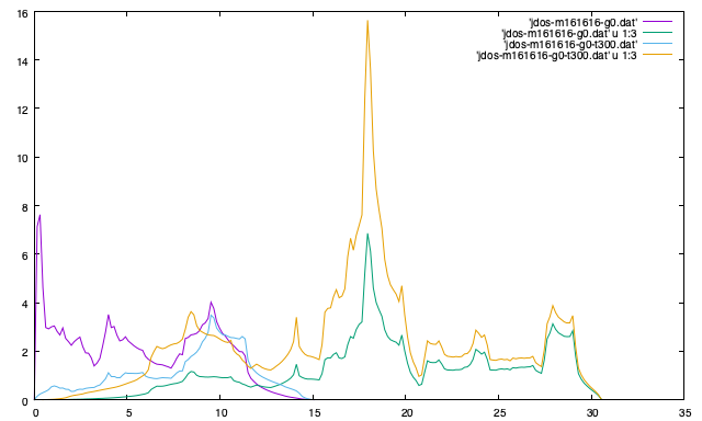
--jdos (JOINT_DOS = .TRUE.)

Two classes of joint density of states (JDOS) are calculated. The result is written into jdos-mxxx-gx(-sx-sdx).dat in \(\text{THz}^{-1}\) (without \((2\pi)^{-1}\)) with respect to frequency in THz (without \(2\pi\)). Frequency sampling points can be specified by --num-freq-points, --freq-pitch (NUM_FREQUENCY_POINTS).

The first column is the frequency, and the second and third columns are the values given as follows, respectively,

\[\begin{split}&D_2^{(1)}(\mathbf{q}, \omega) = \frac{1}{N} \sum_{\lambda',\lambda''} \Delta(-\mathbf{q}+\mathbf{q}'+\mathbf{q}'') \left[\delta(\omega+\omega_{\lambda'}-\omega_{\lambda''}) + \delta(\omega-\omega_{\lambda'}+\omega_{\lambda''}) \right], \\ &D_2^{(2)}(\mathbf{q}, \omega) = \frac{1}{N} \sum_{\lambda',\lambda''} \Delta(-\mathbf{q}+\mathbf{q}'+\mathbf{q}'') \delta(\omega-\omega_{\lambda'} -\omega_{\lambda''}).\end{split}\]

% phono3py --fc2 --dim="2 2 2" --pa="0 1/2 1/2 1/2 0 1/2 1/2 1/2 0" -c POSCAR-unitcell --mesh="16 16 16" --jdos --ga="0 0 0  8 8 8"

When temperatures are specified, two classes of weighted JDOS are calculated. The result is written into jdos-mxxx-gx(-sx)-txxx.dat in \(\text{THz}^{-1}\) (without \((2\pi)^{-1}\)) with respect to frequency in THz (without \(2\pi\)). In the file name, txxx shows the temperature. The first column is the frequency, and the second and third columns are the values given as follows, respectively,

\[\begin{split}&N_2^{(1)}(\mathbf{q}, \omega) = \frac{1}{N} \sum_{\lambda'\lambda''} \Delta(-\mathbf{q}+\mathbf{q}'+\mathbf{q}'') (n_{\lambda'} - n_{\lambda''}) [ \delta( \omega + \omega_{\lambda'} - \omega_{\lambda''}) - \delta( \omega - \omega_{\lambda'} + \omega_{\lambda''})], \\ &N_2^{(2)}(\mathbf{q}, \omega) = \frac{1}{N} \sum_{\lambda'\lambda''} \Delta(-\mathbf{q}+\mathbf{q}'+\mathbf{q}'') (n_{\lambda'}+ n_{\lambda''}+1) \delta( \omega - \omega_{\lambda'} - \omega_{\lambda''}).\end{split}\]

% phono3py --fc2 --dim="2 2 2" --pa="0 1/2 1/2 1/2 0 1/2 1/2 1/2 0" -c POSCAR-unitcell --mesh="16 16 16" --jdos --ga="0 0 0  8 8 8" --ts=300

This is an example of Si-PBEsol.

Sampling frequency for distribution functions

--num-freq-points, --freq-pitch (NUM_FREQUENCY_POINTS)

For spectrum like calculations of imaginary part of self energy and JDOS, number of sampling frequency points is controlled by --num-freq-points or --freq-pitch.

Mode-Gruneisen parameter from 3rd order force constants

--gruneisen (GRUNEISEN = .TRUE.)

Mode-Gruneisen-parameters are calculated from fc3.

Mesh sampling mode:

% phono3py --fc3 --fc2 --dim="2 2 2" -v --mesh="16 16 16" -c POSCAR-unitcell --nac --gruneisen

Band path mode:

% phono3py --fc3 --fc2 --dim="2 2 2" -v -c POSCAR-unitcell --nac --gruneisen --band="0 0 0  0 0 1/2"

File I/O

--fc2 (READ_FC2 = .TRUE.)

Read 2nd order force constants from fc2.hdf5.

--fc3 (READ_FC3 = .TRUE.)

Read 3rd order force constants from fc3.hdf5.

--write-gamma (WRITE_GAMMA = .TRUE.)

Imaginary parts of self energy at harmonic phonon frequencies \(\Gamma_\lambda(\omega_\lambda)\) are written into file in hdf5 format. The result is written into kappa-mxxx-gx(-sx-sdx).hdf5 or kappa-mxxx-gx-bx(-sx-sdx).hdf5 with --bi option. With --sigma and --sigma-cutoff options, -sx and --sdx are inserted, respectively, in front of .hdf5.

--read-gamma (READ_GAMMA = .TRUE.)

Imaginary parts of self energy at harmonic phonon frequencies \(\Gamma_\lambda(\omega_\lambda)\) are read from kappa file in hdf5 format. Initially the usual result file of kappa-mxxx(-sx-sdx).hdf5 is searched. Unless it is found, it tries to read kappa file for each grid point, kappa-mxxx-gx(-sx-sdx).hdf5. Then, similarly, kappa-mxxx-gx(-sx-sdx).hdf5 not found, kappa-mxxx-gx-bx(-sx-sdx).hdf5 files for band indices are searched.

--write-gamma-detail (WRITE_GAMMA_DETAIL = .TRUE.)

Each q-point triplet contribution to imaginary part of self energy is written into gamma_detail-mxxx-gx(-sx-sdx).hdf5 file. Be careful that this is large data.

In the output file in hdf5, following keys are used to extract the detailed information.

gamma_detail for --ise	(temperature, sampling frequency point, symmetry reduced set of triplets at a grid point, band1, band2, band3) in THz (without \(2\pi\))
gamma_detail for --br	(temperature, symmetry reduced set of triplets at a grid point, band1, band2, band3) in THz (without \(2\pi\))
mesh	Numbers of sampling mesh along reciprocal axes.
frequency_point for --ise	Sampling frequency points in THz (without \(2\pi\)), i.e., \(\omega\) in \(\Gamma_\lambda(\omega)\)
temperature	(temperature,), Temperatures in K
triplet	(symmetry reduced set of triplets at a grid point, 3), Triplets are given by the grid point indices (see below).
weight	(symmetry reduced set of triplets at a grid point,), Weight of each triplet to imaginary part of self energy

Imaginary part of self energy (linewidth/2) is recovered by the following script:

import h5py
import numpy as np

gd = h5py.File("gamma_detail-mxxx-gx.hdf5")
temp_index = 30 # index of temperature
temperature = gd['temperature'][temp_index]
gamma_tp = gd['gamma_detail'][:].sum(axis=-1).sum(axis=-1)
weight = gd['weight'][:]
gamma = np.dot(weight, gamma_tp[temp_index])

For example, for --br, this gamma gives \(\Gamma_\lambda(\omega_\lambda)\) of the band indices at the grid point indicated by \(\lambda\) at the temperature of index 30. If any bands are degenerated, those gamma in kappa-mxxx-gx(-sx-sdx).hdf5 or gamma-mxxx-gx(-sx-sdx).hdf5 type file are averaged, but the gamma obtained here in this way are not symmetrized. Apart from this symmetrization, the values must be equivalent between them.

To understand each contribution of triptle to imaginary part of self energy, reading phonon-mxxx.hdf5 is useful (see --write-phonon (WRITE_PHONON = .TRUE.)). For example, phonon triplets of three phonon scatterings are obtained by

import h5py
import numpy as np

gd = h5py.File("gamma_detail-mxxx-gx.hdf5", 'r')
ph = h5py.File("phonon-mxxx.hdf5", 'r')
gp1 = gd['grid_point'][()]
triplets = gd['triplet'][:] # Sets of (gp1, gp2, gp3) where gp1 is fixed
mesh = gd['mesh'][:]
grid_address = ph['grid_address'][:]
q_triplets = grid_address[triplets] / mesh.astype('double')
# Phonons of triplets[2]
phonon_tp = [(ph['frequency'][i], ph['eigenvector'][i]) for i in triplets[2]]
# Fractions of contributions of tripltes at this grid point and temperture index 30
gamma_sum_over_bands = np.dot(weight, gd['gamma_detail'][30].sum(axis=-1).sum(axis=-1).sum(axis=-1))
contrib_tp = [gd['gamma_detail'][30, i].sum() / gamma_sum_over_bands for i in range(len(weight))]
np.dot(weight, contrib_tp) # is one

--write-phonon (WRITE_PHONON = .TRUE.)

Phonon frequencies, eigenvectors, and grid point addresses are stored in phonon-mxxx.hdf5 file. –pa and –nac may be required depending on calculation setting.

% phono3py --fc2 --dim="2 2 2" --pa="0 1/2 1/2 1/2 0 1/2 1/2 1/2 0" --mesh="11 11 11" -c POSCAR-unitcell --nac --write-phoonon

Contents of phonon-mxxx.hdf5 are watched by:

In [1]: import h5py

In [2]: ph = h5py.File("phonon-m111111.hdf5", 'r')

In [3]: list(ph)
Out[3]: ['eigenvector', 'frequency', 'grid_address', 'mesh']

In [4]: ph['mesh'][:]
Out[4]: array([11, 11, 11], dtype=int32)

In [5]: ph['grid_address'].shape
Out[5]: (1367, 3)

In [6]: ph['frequency'].shape
Out[6]: (1367, 6)

In [7]: ph['eigenvector'].shape
Out[7]: (1367, 6, 6)

The first axis of ph['grid_address'], ph['frequency'], and ph['eigenvector'] corresponds to the number of q-points where phonons are calculated. Here the number of phonons may not be equal to product of mesh numbers (\(1367 \neq 11^3\)). This is because all q-points on Brillouin zone boundary are included, i.e., even if multiple q-points are translationally equivalent, those phonons are stored separately though these phonons are physically equivalent within the equations employed in phono3py. Here Brillouin zone is defined by Wigner–Seitz cell of reciprocal primitive basis vectors. This is convenient to categorize phonon triplets into Umklapp and Normal scatterings based on the Brillouin zone.

--read-phonon (READ_PHONON = .TRUE.)

Phonon frequencies, eigenvectors, and grid point addresses are read from phonon-mxxx.hdf5 file and the calculation is continued using these phonon values. This is useful when we want to use fixed phonon eigenvectors that can be different for degenerate bands when using different eigenvalue solvers or different CPU architectures. –pa and –nac may be required depending on calculation setting.

% phono3py --fc2 --fc3 --dim="2 2  2" --pa="0 1/2 1/2 1/2 0 1/2 1/2 1/2 0" --mesh="11 11 11" -c POSCAR-unitcell --nac --read-phoonon --br

--write-pp (WRITE_PP = .TRUE.) and --read-pp (READ_PP = .TRUE.)

Phonon-phonon (ph-ph) intraction strengths are written to and read from pp-mxxx-gx.hdf5. This works only in the calculation of lattice thermal conductivity, i.e., usable only with --br or --lbte. The stored data are different with and without specifying --full-pp option. In the former case, all the ph-ph interaction strengths among considered phonon triplets are stored in a simple manner, but in the later case, only necessary elements to calculate collisions are stored in a complicated way. In the case of RTA conductivity calculation, in writing and reading, ph-ph interaction strength has to be stored in memory, so there is overhead in memory than usual RTA calculation.

% phono3py --fc2 --fc3 --dim="2 2 2" --pa="0 1/2 1/2 1/2 0 1/2 1/2 1/2 0" --mesh="11 11 11" -c POSCAR-unitcell --nac --write-pp --br --gp=1

% phono3py --fc2 --dim="2 2 2" --pa="0 1/2 1/2 1/2 0 1/2 1/2 1/2 0" --mesh="11 11 11" -c POSCAR-unitcell --nac --read-pp --br --gp=1

--hdf5-compression (command option only)

Most of phono3py HDF5 output file is compressed by default with the gzip compression filter. To avoid compression, --hdf5-compression=None has to be set. Other filters (lzf or integer values of 0 to 9) may be used, see h5py documentation (http://docs.h5py.org/en/stable/high/dataset.html#filter-pipeline).

-o (command option only)

This modifies default output file names to write.

Using this option, output file names are slightly modified. For example, with -o iso, a file name kappa-m191919.hdf5 is changed to kappa-m191919.iso.hdf5.

This rule is applied to

• fc3.hdf5

• fc2.hdf5

• kappa-xxx.hdf5

• phonon-xxx.hdf5

• pp-xxx.hdf5

• disp_fc3.yaml

• disp_fc2.yaml

• gamma_detail-xxx.hdf5 (write only)

-i (command option only)

This modifies default input file names to read.

Using this option, input file names are slightly modified. For example, specifying -i iso --fc3, a file name fc3.iso.hdf5 is read instead of fc3.hdf5.

This rule is applied to

• fc3.hdf5

• fc2.hdf5

• kappa-xxx.hdf5

• phonon-xxx.hdf5

• pp-xxx.hdf5

• disp_fc3.yaml

• disp_fc2.yaml

--io (command option only)

This modifies default input and output file names.

This is equivalent to setting -i and -o simultaneously.